Workflow
The following steps give a causal analysis with DoubleML PySpark its structure. Each step is explained and shown on one running example: a coupon campaign of an online retailer. For effects by customer group and the decision who should get the coupon, see the business example.
0. Problem formulation
A retailer sent a coupon to part of its customers. Treatment: the coupon. Outcome: revenue per customer in the following 30 days. Question: how much additional revenue does the coupon cause? Each coupon costs 3 USD and 35 % of additional revenue is profit, so the coupon pays for itself above 8.57 USD.
The coupon was not sent at random. The CRM favours active customers, app users and high spenders, who buy a lot anyway. These characteristics influence both who gets the coupon and how much the customer spends, so they are confounders:
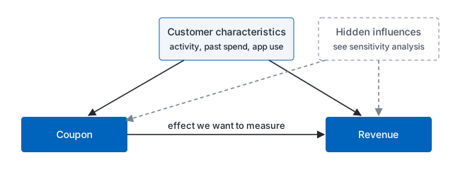
We therefore include these characteristics as covariates. Step 8 shows how robust the result is to influences we did not observe.
1. Data backend
We start the Spark session and load the data. On Databricks the session already exists. The
dataset is simulated, so true_effect shows the correct answer, which real data would not have.
With your own table, add a unique ID column if there is none, for example with
monotonically_increasing_id(): DoubleML uses it to align the predictions across the folds.
from pyspark.sql import SparkSession
from pyspark.sql import functions as F

from doubleml_pyspark.datasets import make_coupon_data

spark = SparkSession.getActiveSession() or SparkSession.builder.getOrCreate()

df, covariates = make_coupon_data(spark, n_obs=20_000, seed=42)
print(covariates)
df.limit(5).toPandas()
['tenure_months', 'log_past_spend', 'visits_90d', 'discount_share', 'app_user', 'region_south', 'region_east', 'region_west']
| ID | tenure_months | log_past_spend | visits_90d | discount_share | app_user | region_south | region_east | region_west | segment | coupon | basket_value_30d | true_effect | |
|---|---|---|---|---|---|---|---|---|---|---|---|---|---|
| 0 | 0 | 96.0 | 5.562929 | 6.0 | 0.091933 | 0.0 | 0.0 | 1.0 | 0.0 | regular | 0.0 | 45.542386 | 3.873781 |
| 1 | 1 | 79.0 | 5.624077 | 2.0 | 0.162034 | 0.0 | 0.0 | 0.0 | 0.0 | regular | 0.0 | 17.317332 | 2.121261 |
| 2 | 2 | 30.0 | 5.330364 | 12.0 | 0.579146 | 0.0 | 0.0 | 0.0 | 0.0 | bargain_hunter | 0.0 | 52.940097 | 11.649484 |
| 3 | 3 | 25.0 | 6.608067 | 4.0 | 0.216143 | 1.0 | 0.0 | 1.0 | 0.0 | vip | 0.0 | 47.888208 | 0.005134 |
| 4 | 4 | 77.0 | 6.131646 | 1.0 | 0.273976 | 1.0 | 0.0 | 0.0 | 0.0 | regular | 0.0 | 33.960504 | 2.760877 |
The field map declares which column plays which role.
data_field_map = {
    "id_column": "ID",
    "outcome": "basket_value_30d",
    "treatment": "coupon",
    "covariates": covariates,
}
2. Causal model
| Model | Class | Treatment | Assumption |
|---|---|---|---|
| Interactive regression model (IRM) | DoubleMLIRM |
binary | the effect may differ between customers |
| Partially linear regression (PLR) | DoubleMLPLR |
continuous or binary | one effect for everyone |
The coupon is binary and will not work equally for everyone, so we choose IRM. For a price or a
discount level, PLR is the natural choice. The target parameter is the average effect over all
customers ("ATE"), or over those who received the coupon ("ATT").
from doubleml_pyspark.irm import DoubleMLIRM

dml = DoubleMLIRM(
    data_schema=df.schema,
    data_field_map=data_field_map,
    target_parameter="ATE",
)
PLR is set up the same way:
from doubleml_pyspark.plm import DoubleMLPLR

dml_plr = DoubleMLPLR(data_schema=df.schema, data_field_map=data_field_map)
3. Machine learning methods
Any Spark ML estimator can be used. Match the model to the variable: classifiers for binary variables, regressors for continuous ones. IRM needs three models:
ml_m: who receives the treatment (classifier)ml_g0: outcome without treatment (regressor)ml_g1: outcome with treatment (regressor)
PLR needs two regressors: ml_l for the outcome and ml_m for the treatment.
Here we use gradient boosted trees with few rounds, so that the example runs quickly. On your own data, more rounds or tuning (step 5) are usually better.
from pyspark.ml.classification import GBTClassifier
from pyspark.ml.regression import GBTRegressor

ml_models = {
    "ml_m": GBTClassifier(maxIter=10, maxDepth=5, stepSize=0.3, seed=42),
    "ml_g0": GBTRegressor(maxIter=10, maxDepth=5, stepSize=0.3, seed=42),
    "ml_g1": GBTRegressor(maxIter=10, maxDepth=5, stepSize=0.3, seed=42),
}
4. Cross-fitting
Each model predicts only for customers it was not trained on, which removes the overfitting
bias. Five folds are the usual choice, for very large data two or three are often enough and
cost less compute. Here we use two. With n_rep above 1 you get several repetitions,
and fit() takes one at a time.
from doubleml_pyspark.utils import kfold_split

splits = kfold_split(df, n_folds=2, n_rep=1, shuffle=True, seed=42)
5. Hyperparameter tuning
Tuning is optional, but can improve the estimate with flexible models. It costs extra compute,
so we show it without running it here. Tune on one split or a sample, then pass the result to
fit() in place of ml_models. See Optuna tuning for more.
def gbt_space(trial):
    return {
        "maxDepth": trial.suggest_int("maxDepth", 3, 6),
        "maxIter": trial.suggest_int("maxIter", 10, 40),
        "stepSize": trial.suggest_float("stepSize", 0.05, 0.3, log=True),
    }

best_models = dml.tune_ml_models(
    spark_session=spark,
    data_split=splits[0][0],  # repetition 0, fold 0
    ml_models=ml_models,
    ml_param_space=dict.fromkeys(ml_models, gbt_space),
    optuna_settings={"n_trials": 10, "gc_after_trial": True},
)
6. Estimation
fit() runs the cross-fitting and computes the effect. On classic clusters, df.cache() before
the fit saves compute. Serverless compute does not support cache(), see the
business example for how to store the data as
a Delta table instead.
dml.fit(spark_session=spark, kfold_split=splits[0], ml_models=ml_models)

print("effect:        ", dml.coef)
print("standard error:", dml.se)
print(dml.summary)
effect:         [6.50926036]
standard error: [0.21564643]
           coef   std err          t  P>|t|     2.5 %   97.5 %
coupon  6.50926  0.215646  30.184875    0.0  6.086601  6.93192
7. Inference
Now we interpret the result. For comparison we add what a simple comparison of customers with and without coupon would have said, and the true effect.
means = df.groupBy("coupon").agg(F.avg("basket_value_30d")).toPandas().set_index("coupon").iloc[:, 0]
naive = means[1.0] - means[0.0]
true_effect = df.agg(F.avg("true_effect")).first()[0]
break_even = 3.0 / 0.35

print(dml.confint())
print(f"simple comparison {naive:.2f} USD")
print(f"DoubleML          {dml.coef[0]:.2f} USD")
print(f"true effect       {true_effect:.2f} USD")
print(f"break-even        {break_even:.2f} USD")
           2.5 %   97.5 %
coupon  6.086601  6.93192
simple comparison 19.48 USD
DoubleML          6.51 USD
true effect       6.16 USD
break-even        8.57 USD
The simple comparison is far too high and suggests that the campaign pays for itself. DoubleML is close to the true effect, and its confidence interval lies below break-even: sent like this, the campaign loses money.
8. Sensitivity analysis
What if we missed a confounder? cf_y and cf_d set how much a hidden influence could explain of
the outcome and of the treatment. The summary shows the resulting range for the effect. The
robustness value (RV) says how strong a hidden influence would have to be to reduce the effect to
zero: a high value means the conclusion is hard to overturn.
A practical starting point is to compare with the observed covariates: how much do the strongest ones explain?
dml.sensitivity_analysis(cf_y=0.03, cf_d=0.03)
print(dml.sensitivity_summary)
================== Sensitivity Analysis ==================

------------------ Scenario          ------------------
Significance Level: level=0.95
Sensitivity parameters: cf_y=0.03; cf_d=0.03, rho=1.0

------------------ Bounds with CI    ------------------
        CI lower  theta lower    theta  theta upper  CI upper
coupon  5.339378     5.696266  6.50926     7.322254  7.676204

------------------ Robustness Values ------------------
        H_0     RV (%)    RVa (%)
coupon  0.0  21.594941  20.410729
Next steps
- Business example: effects by customer group, charts and who should get the coupon
- API reference
- Chernozhukov, V., Chetverikov, D., Demirer, M., Duflo, E., Hansen, C., Newey, W., & Robins, J. (2018). Double/debiased machine learning for treatment and structural parameters. The Econometrics Journal, 21(1), C1-C68.